Today, the most powerful large language model is GPT-4, developed by OpenAI, which has even outperformed the average human in many tests.

What’s the secret behind GPT-4? Although OpenAI has not disclosed the model’s specifics, they have scaled the GPT-3 model 100 times to GPT-4, totaling 1.76 trillion parameters. However, training such a large-scale dense model is highly expensive considering the cost. AI researchers have believed that OpenAI has adopted the MoE (Mixture of Experts) approach in its architecture, allowing for increased scale while reducing the consumption of computational resources.

Transformer

Let’s first review the basics of the Transformer model:

The transformer architecture consists of an encoder and a decoder. Both the encoder and decoder are composed of multiple layers. In Figure 1, the left part is the encoder, and the decoder is on the right side. Each layer in the encoder and the decoder typically contains two main components: multi-head self-attention and point-wise feed-forward networks. The encoder processes the input sequences while the decoder generates new sentences.

1. Transformer architecture (Source: Ashish Vaswani, 2017).

Current large language models (LLMs) generally use decoder-only transformers since the models are usually used for autoregression generation tasks. GPT and LLAMA are prominent examples of decoder-only transformers. Using these transformers allows the model to process all previously generated tokens during the generation procedure, facilitating the autoregressive nature of the task. They have demonstrated the effectiveness of decoder-only transformers in language modeling, machine translation, and text generation tasks.

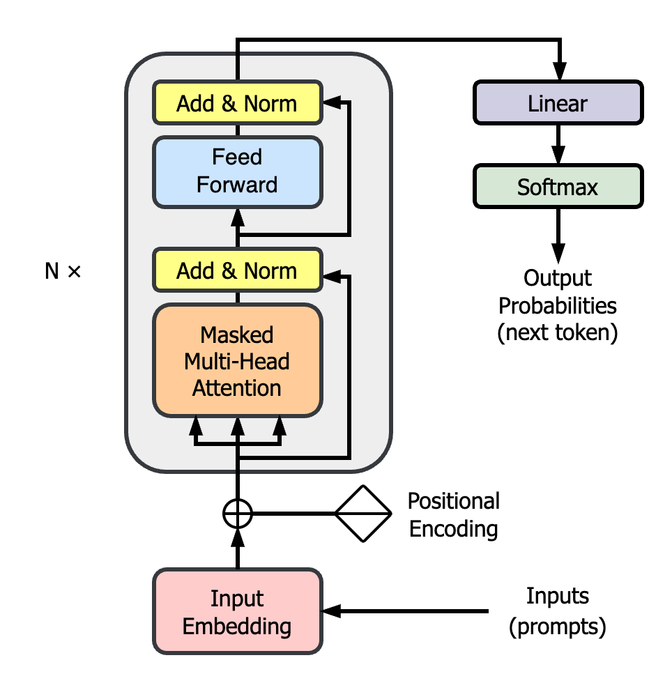
2. Decoder block of the transformer.

The decoder blocks in the model contain point-wise feed-forward networks (FFN) that consist of multiple linear layers and activation functions. These linear layers use text tokens as inputs and turn them into weight information that stores the correlation between these tokens. Given the complexity of text information and the ambiguous relationships between words, activation functions add the ability for the FFN to represent non-linear relations.

3. Compare two types of decoder.

Taking the 70B LLAMA2 model as an example, its FFN layer contains approximately 0.7 billion parameters. Moreover, it comprises 80 hidden layers, making the computational load for each token input during training and inference substantial. Further increasing the parameter count could easily lead to performance bottlenecks. To address this, we need a method that can leverage limited computational resources to improve the performance of LLMs — Mixture of Experts (MoE).

Mixture of Experts (MoE)

What is MoE?

The Mixture of Experts (MoE) in LLMs involves replicating the Feed-Forward Network (FFN) into multiple instances, each serving as a distinct expert. These experts are controlled by a router, which determines the selection of specific experts to process token inputs. The concept of MoE has been proposed for quite some time and has been used in various domains such as computer vision (CV), natural language processing (NLP), and even reinforcement learning (RL). However, it wasn’t until GPT-4 that this idea gradually gained popularity.

There are two types of feed-forward network layers:

• Dense model (Llama) uses all parameters to process inputs every time and requires full-parameter computations.
• Sparse model (Mixtral) only uses a partition of parameters for computations, whereas others are inactivated and not involved in computations. The partial computations will significantly reduce the computing power costs and make processing faster compared to its dense counterpart.

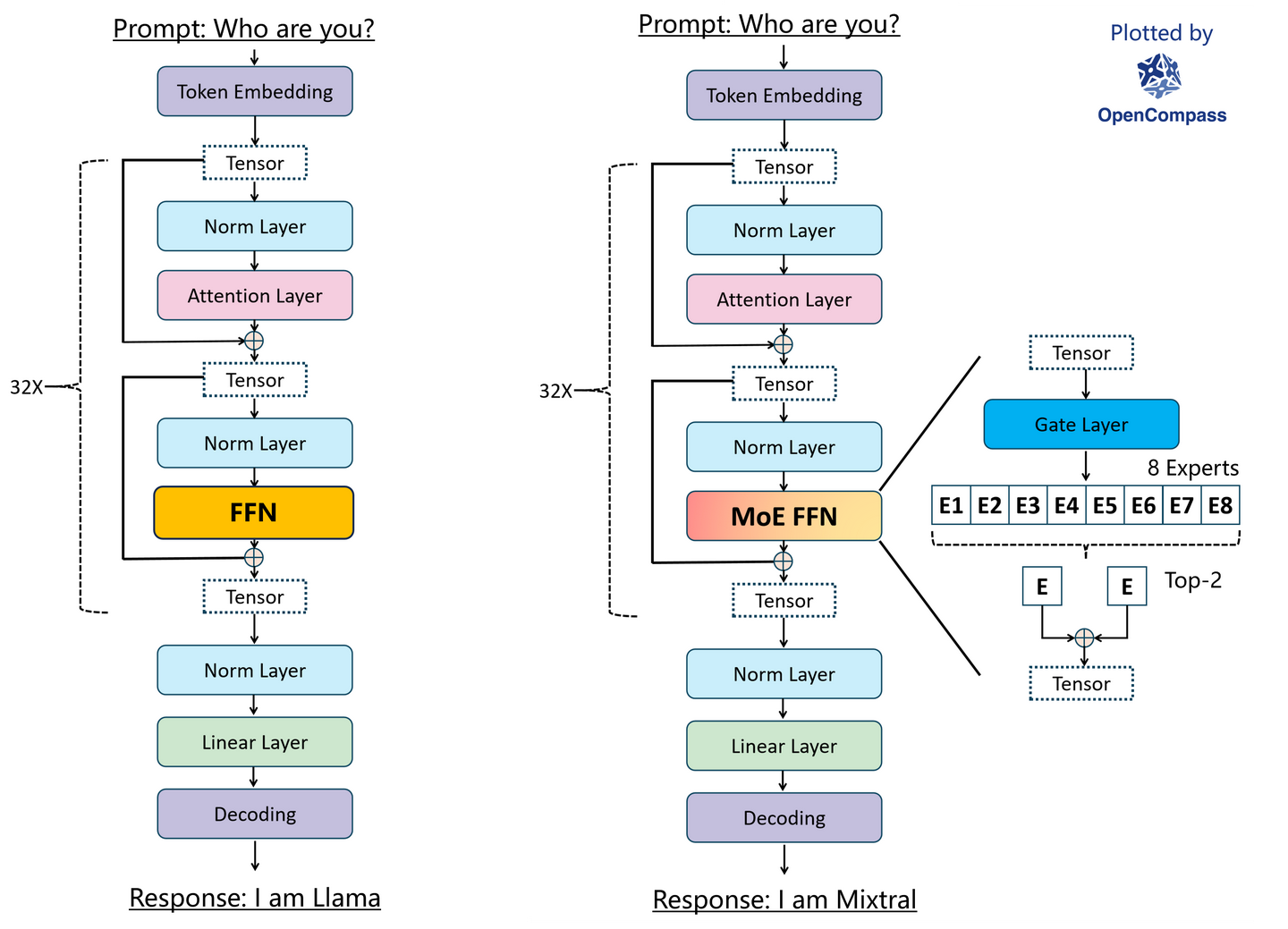
4. Llama dense model vs. Mixtral sparse model

Why we use MoE?

Imagine you are assigning a project to a software team. This team consists of engineers with varying abilities who collaborate to complete tasks. The project manager in this team acts just like the “Router” in MoE. He is responsible for analyzing and planning the project and assigning tasks to the team members. These team members, like the “Experts” in MoE, are responsible for handling different aspects of the project. During this process, each role handles what they are best at. The project manager then integrates the completed tasks to form a cohesive project.

Assuming that there is only one person in this team, a full-stack engineer possessing all the abilities of the multiple experts mentioned earlier, while they might be able to accomplish the same tasks, the compensation they would demand is significantly higher than that of each individual in the team of experts. The team of experts only needs to pay each participating member, whereas a one-person team would require the same payment whether the project is simple or complicated. In terms of efficiency, a team of multiple experts can handle different tasks simultaneously, while a one-person team can only handle one task. Therefore, a team of experts is superior to a one-person team in cost and efficiency.

We find that the expert mechanism is everywhere in various domains. Most individuals excel in specific areas, and people collaborate to accomplish complex tasks. This approach is more efficient than having a jack-of-all-trades handle the tasks.

In a translation task, a multilingual input aligns well with the MoE Sparse models.

When we want to translate a word or a sentence, such as “What is ‘你好’ in English?”, a Dense model would take each word of the sentence as the same input, and then all the parameters of the model would be used to process these inputs and return the corresponding result. The benefit of this approach is that all the useful parameters of the model are engaged in processing the input to obtain the best result. However, most of the parameters involved are not relevant to translating Chinese, which increases the cost of translation and affects the correct translation result. Perhaps we can discuss whether the parameters for processing French in the model help translate Chinese. But evidently, the high-cost information processing in a dense model makes it difficult to find the optimal solution.

5. Translation with a dense model.

When we input the same question into a Sparse model, each word will route and be sent to the corresponding expert. As shown in the figure below, each expert specializes in its language. Therefore, during the translation process, we can more effectively utilize the expertise of the corresponding language experts. For instance, Chinese words are handled by experts specializing in Chinese, while French experts are completely excluded from processing. This reduces unnecessary resource wastage, making this processing mode more efficient compared to the Dense model.

6. Translation with a sparse model.

Researchers from Google have also found experts that specialize in different types of text:

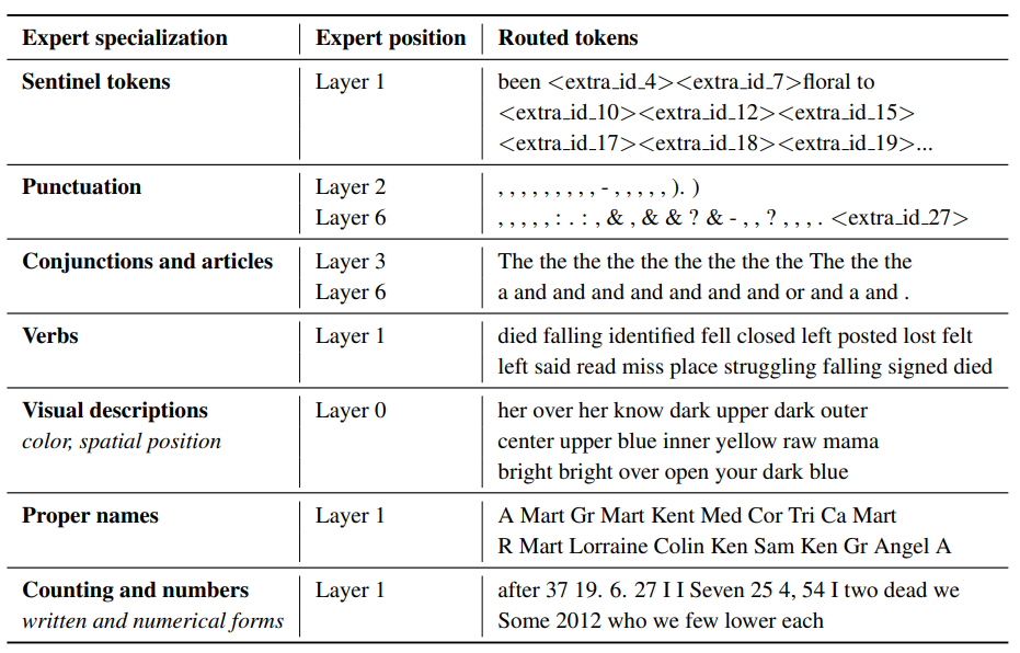
7. Expert specialization (Source: William Fedus, 2022).

How MoE works?

In the implementation of MoE in LLMs, a MoE block consisting of a Router and multiple FFN copies replaces the original FFN layer in the Dense model as Experts. Each of these FFN copies represents an expert.

The FFN layer in the Dense model typically transforms the input embeddings to extract high-level abstractions from the text input, allowing LLM to understand what we intend to say.

The MoE FFN functions similarly to the FFN, transforming input embeddings to better understand text content. However, the MoE’s architecture and pipeline make it more efficient in handling this process.

Router

Routing is a process of choosing experts for each token input. A router or gate layer is a Gating Network $G(x)$ with trainable parameters. It takes input tokens and outputs weights representing the contribution of each expert in processing the input, which also indicates the probability of each expert being selected in the routing process. Typically, we use the Softmax function to ensure these probabilities are distributed with a sum of 1.

Let’s assume we have four experts in a MoE layer, and the router outputs weights of 0.4, 0.3, 0.2, and 0.1 corresponding to each expert when an input token is taken. This means that the expert with a higher weight can better handle the input. In this case, we choose the first two experts with the highest weights to process the input to obtain the best result.

The Gate Network is specified as: \(G_\sigma(x)=Softmax(x\cdot W_g)\) where $x$ is the input data and $W_g$ is the routing weight.

There are some common routing methods:

1. Token choice routing (Top-K)

   Top-k routing is commonly used in many MoE LLMs, it allows each token to choose $k$ experts with the highest probability ($1 ≤ k ≤ n$) where $n$ is the total number of experts.

   

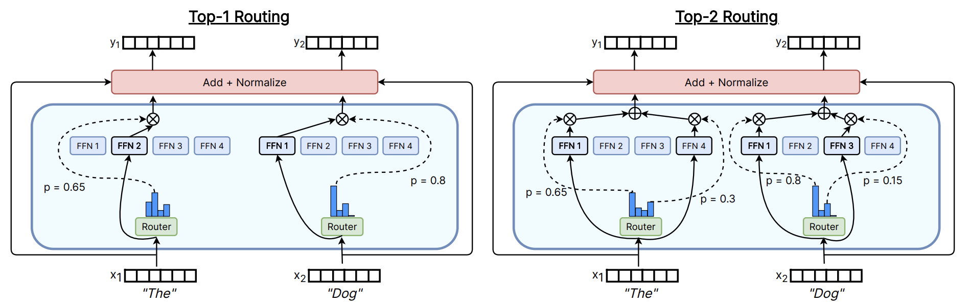
   8. Top-K routing (k = 1, 2) (Source: William Fedus, 2022).

   After routing each token to the selected experts, the output embedding from the experts are multiplied by their corresponding routing weights. These multiplications are then summed up to produce the final results.

2. Expert choice routing

   Instead of each token choosing experts in routing, each expert can also choose the top-k tokens for processing. This method guarantees even load balancing for every expert during training.

   

   9. Expert choice routing (Source: William Fedus, 2022).

Experts

Expert models are made up of several feed-forward networks with the same shapes. These experts can be viewed as multiple copies of the FFN in the dense model. In most cases, each expert FFN does not have as many weight parameters as the FFN in the Dense model. Two types of feed-forward networks are used commonly in LLMs:

• LlaMA-based SwiGLU FFN:
  • $SwiGLU(x, W, V, b, c) = Swish\beta(x\cdot W + b) \otimes (x\cdot V + c)$
  • $Swish(\beta=1)(x) = SiLU(x) = x\cdot \sigma (x)$
  • $FFNSwiGLU(x, W_1, W_2, W_3) = (SiLU(x\cdot W_1) \otimes x\cdot W_3) \cdot W_2$

      class SwiGLUFFN(nn.Module):
      def __init__(self, hidden_dim: int, intermediate_dim: int):
          super().__init__()
          self.w1 = nn.Linear(hidden_dim, intermediate_dim, bias=False)
          self.w3 = nn.Linear(hidden_dim, intermediate_dim, bias=False)
          self.w2 = nn.Linear(intermediate_dim, hidden_dim, bias=False)
                
          self.act_fn = nn.SiLU()
                
      def forward(self, x: torch.Tensor) -> torch.Tensor:
          h = self.act_fn(self.w1(x)) * self.w3(x)
          h = self.w2(h)
          return h
    

• GPT-based FFN
  • $FFN_{GELU}(x, W_1, W_2) = GELU(x\cdot W_1)\cdot W_2$

    class VanillaFFN(nn.Module):
    	def __init__(self, hidden_dim: int, intermediate_dim: int):
    		super().__init__()
    		self.w1 = nn.Linear(hidden_dim, intermediate_dim, bias=False)
    		self.w2 = nn.Linear(intermediate_dim, hidden_dim, bias=False)
      		
    		self.act_fn = nn.GELU()
      		
    	def forward(self, x: torch.Tensor) -> torch.Tensor:
    		h = self.act_fn(self.w1(x)) 
    		h = self.w2(h)
    		return h
  

10. On the left, the modified FFN layer with SwiGLU; On the right, the FFN layer of the original transformer (Source: Deci, 2024).

Pipeline

When the experts are chosen by the router, the input data is sent to the selected expert FFN layers. The experts not chosen in the routing will remain inactivate.

During the inference and training, only portion of experts are activated simultaneously, and most parameters are not used. The overall pipeline will be:

where $G(x)$ is the Gate Net and $E_i(x)$ is the Expert FFN.

When an input token $x$ is sent to the Gate Net, $G(x)_i$ outputs the probability of choosing the $i$-th expert. In Top-k routing, only $k$ experts are selected for each token. in this case, $G(x)_i$ equals zero if the $i$-th expert is not selected, thereby deactivating the parameters of the unselected expert. This mechanism significantly reduces computation costs.

The outputs of these $k$ experts are multiplied by their corresponding routing weight and then combined to form the final output.

The implementation of MoE layer:

# Refer to Mixtral's Implementation
class SparseMoeBlock(nn.Module):
	def __init__(self, config):
		super().__init__():
		self.hidden_dim = config.hidden_size
		self.intermediate_dim = config.intermediate_size
		self.num_experts = config.num_experts
		self.top_k = config.num_experts_per_tok
		
		# router
		self.gate_net = nn.Linear(self.hidden_dim, self.num_experts, bias=False)
		
		# experts
		self.experts = nn.ModuleList([FFN(self.hidden_dim, self.intermediate_dim) for _ in range(self.num_experts)])
		
	def forward(self, x: torch.Tensor) -> torch.Tensor:
		batch_size, seq_len, hidden_dim = x.shape
		x = x.view(-1, hidden_dim)
    # router_logits: (batch * sequence_length, n_experts)
    router_logits = self.gate_net(x)

    routing_weights = F.softmax(router_logits, dim=1, dtype=torch.float)
    routing_weights, selected_experts = torch.topk(routing_weights, self.top_k, dim=-1)
    routing_weights = routing_weights.to(x.dtype)
    
    # initialize final output
    y = torch.zeros(
        (batch_size * seq_len, hidden_dim), dtype=x.dtype, device=x.device
    )
    
    # One hot encode the selected experts to create an expert mask
    # this will be used to easily index which expert is going to be sollicitated
    expert_mask = torch.nn.functional.one_hot(selected_experts, num_classes=self.num_experts).permute(2, 1, 0)
    
    # Loop over all available experts in the model and perform the computation on each expert
    for expert_idx in range(self.num_experts):
	    expert_layer = self.experts[expert_idx]
	    idx, top_x = torch.where(expert_mask[expert_idx])
	
	    if top_x.shape[0] == 0:
	        continue
	
	    # in torch it is faster to index using lists than torch tensors
	    top_x_list = top_x.tolist()
	    idx_list = idx.tolist()
	
	    # Index the correct hidden states and compute the expert hidden state for
	    # the current expert. We need to make sure to multiply the output hidden
	    # states by `routing_weights` on the corresponding tokens (top-1 and top-2)
	    h = x[None, top_x_list].reshape(-1, hidden_dim)
	    h_out = expert_layer(x) * routing_weights[top_x_list, idx_list, None]
	
	    # However `index_add_` only support torch tensors for indexing so we'll use
	    # the `top_x` tensor here.
	    y.index_add_(0, top_x, h_out.to(x.dtype))
        
		y = y.reshape(batch_size, seq_len, hidden_dim)
		return y

Mixtral

Mixtral is an open-source MoE LLM model built on the base of the Mistral model.

As shown in the figure 4, the Mixtral shares a similar architecture to the Llama model. The only difference is that the Mixtral model replaces the FFN layer with the MoE FFN layer. It applies Top-k routing and adopts SwiGLU for its expert FFNs

Accelerate MoE

Parallelism

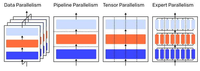
11. Concept of parallelism.

Data Parallelism involves processing a batch of data across different devices in parallel, with each device holding a complete copy of the model. After the forward propagation, the gradient is gathered and updated.

Model Parallelism, on the other hand, involves distributing different model parameters (layers, components) across different devices to process a batch of data.

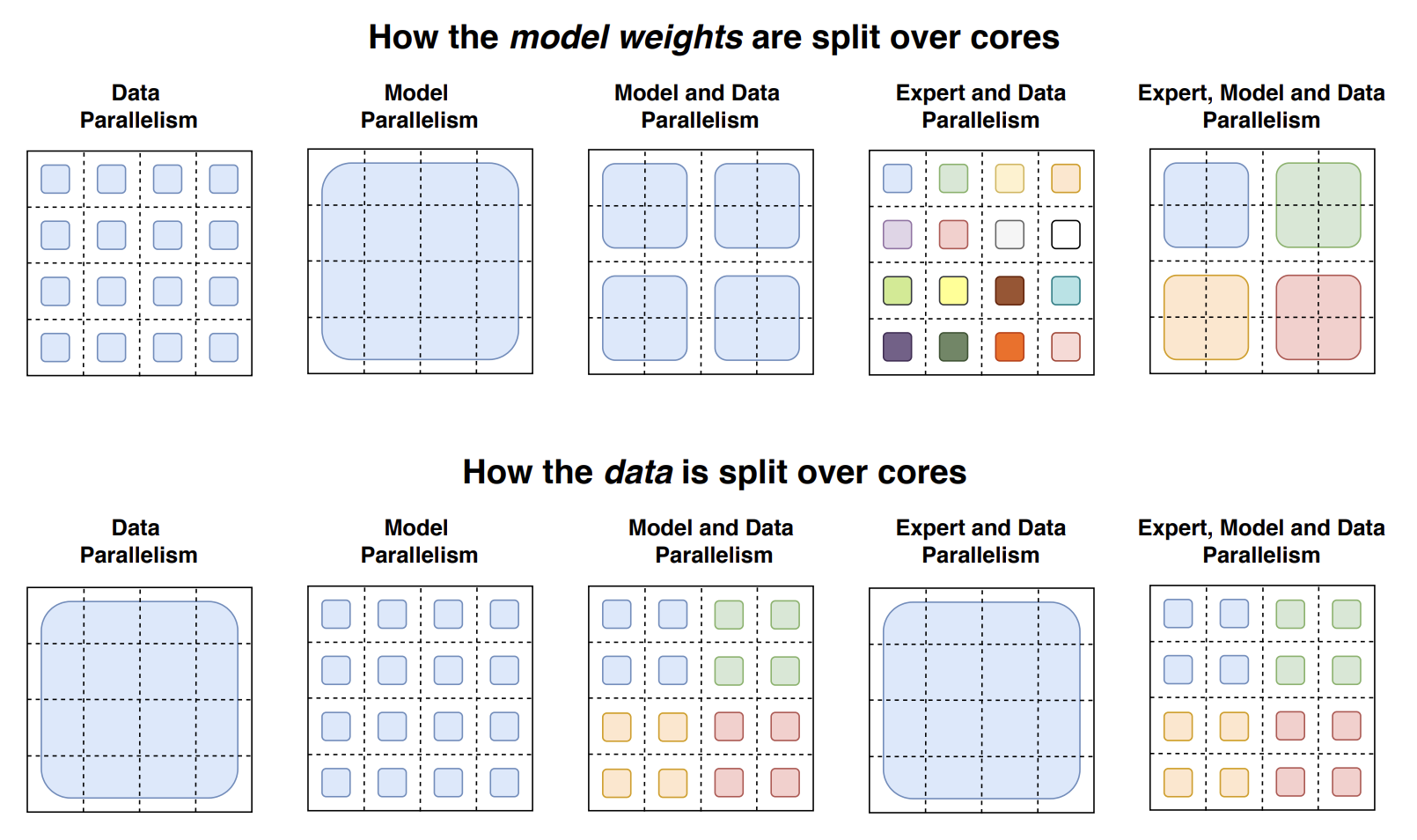
12. How model weights and data is organized over cores (Source: William Fedus, 2021).

Here’s a brief review of the various parallelism methods:

Data Parallelism

As shown in the figure 12, the model weights are copied and distributed over cores. Furthermore, the data is a complete block over cores, which means the data is updated within a single batch over all cores.

Model Parallelism

In contrast to data parallelism, model parallelism involves distributing an entire model across all cores. This means each core will only maintain a portion of the model’s weights, while the same batch of data is duplicated and sent to these cores for computation. Because the model weights on each core are different, communication with other cores is required after each computing, leading to a very high communication cost.

Expert Parallelism

The original routing mechanism would only allocate different experts within the current core. Expert parallelism allows the router to send the token to the experts from other cores, adding cross-core communication between experts.

DeepSpeed

With DeepSpeed-MoE, each expert can be sliced and placed on different devices, leveraging the concept of tensor parallelism across the MoE expert model just like the model parallelism on the dense FFN model. As a result, expert slicing fully utilizes the memory bandwidth on the GPU.

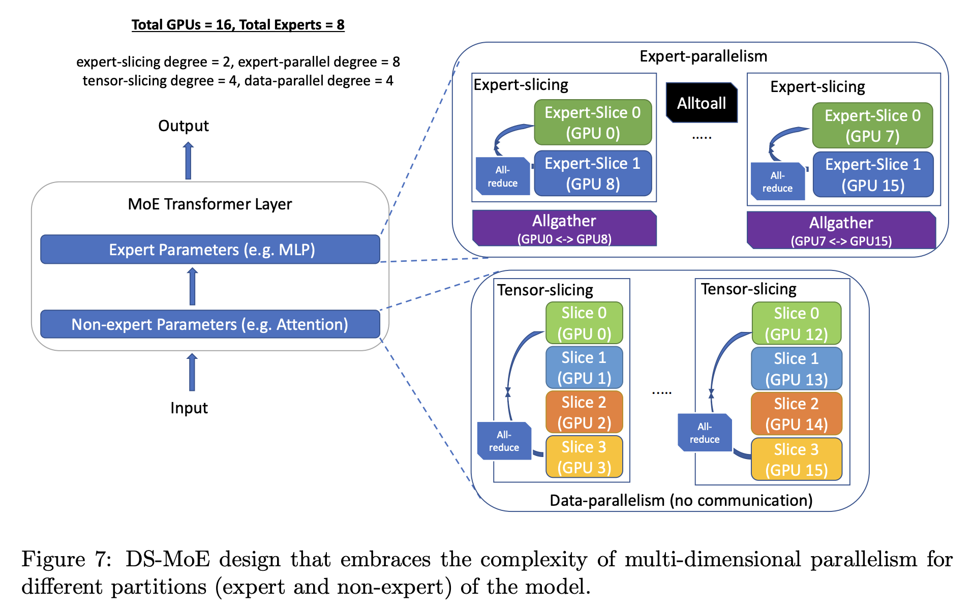
13. DeepSpeed-MoE (Source: Samyam Rajbhandar, 2021).

Grouped GeMM

Let’s delve into the Mixture of Experts (MoE) process from the perspective of matrix multiplication operations.

In the implementation of the MoE layer, we employ the conventional General Matrix Multiplication (GeMM): $x(m, k) @ w(k, n) → y(m, n)$ to compute output of each expert.

Given that there are $n$ experts, the final output of experts is computed by performing GeMM $n$ times in a loop.

$e_1$: $x_1(bs, m_1, k) @ w_1^1(k, 4k) @ w_1^2(4k, k) → y_1(bs, m_1, k)$

$e_2$: $x_2(bs, m_2, k) @ w_2^1(k, 4k) @ w_2^2(4k, k) → y_2(bs, m_2, k)$

…

$e_n$: $x_n(bs, m_n, k) @ w_n^1(k, 4k) @ w_n^2(4k, k) → y_n(bs, m_n, k)$

where $bs$ represents the batch size, $m_i$ denotes the token length of each expert, (please note that $m$ is not the same for all experts), and $k$ indicates the hidden dimension.

The final output of the experts will be represented as $[y_1, …, y_n]$.

To accelerate MoE model on a single device. it becomes essential to compute the matrix multiplication for MoE in parallel. Assuming that all the token lengths $m$ for experts are identical ($m_1 = m_2 = … = m_n$), we can then apply batched GeMM for the computation of MoE with $n$ experts.

Final output: $x(n, bs * m, k) @ w_1(k, 4k) @ w_2(4k, k) → y(n, bs * m, k)$

However, in practical scenarios, the token length for each expert varies. To address this, we need apply zero-padding and drop tokens to align tokens and use batched GeMM.

14. Grouped GeMM is similar to the idea in MegaBlocks (Source: Gale, Trevor, 2023).

Grouped GeMM is introduced to apply the batched matrix multiplication on variable-sized inputs. In the MoE setting, each expert receives tokens with different lengths. To enable parallel matrix multiplication for all experts, Grouped GeMM is designed to partition the large matrix multiplications with distinct sizes into multiple small GeMMs with the same size through tiling decomposition. Subsequently, the large matrix multiplication can be executed by simultaneously computing all small matrix multiplications across all computing units. Through this approach, Grouped GeMM significantly reduces the computational time compared to the sequential single-stream calculation for experts and saturates the utilization of the computing device.

15. Grouped GeMM is used for matrix multiplications by the MoE experts of Figure 14C

References

1. Vaswani, Ashish, et al. “Attention Is All You Need.” NeurIPS (2017).
2. Fedus, William, et al. “Switch transformers: Scaling to trillion parameter models with simple and efficient sparsity.” JMLR (2022).
3. Rajbhandari, Samyam, et al. “Deepspeed-moe: Advancing mixture-of-experts inference and training to power next-generation ai scale.” PMLR (2022).
4. Fedus, William, et al. “A review of sparse expert models in deep learning.” arXiv preprint (2022).
5. Zhou, Yanqi, et al. “Mixture-of-experts with expert choice routing.” NeurIPS (2022).
6. Dai, A., and Nan Du. “More efficient in-context learning with GlaM.” Google Research Blog (2023).
7. Jiang, Albert Q., et al. “Mixtral of experts.” arXiv preprint (2024).
8. Gale, Trevor, et al. “Megablocks: Efficient sparse training with mixture-of-experts.” MLSys (2023).