In the real world, many problems can be formed through Reinforcement Learning(RL). A typical RL problem generally consists of an agent that makes the decision and the environment where the agent is surrounded. This post will go over some important basics from Sutton and Button’s Reinforcement Learning book and introduce several of the classic RL approaches.
Markov Decision Process
How to mathematically formulate an RL problem. From this, we introduce a concept called Markov Decision Process(MDP). With the Markov Property of state transition, we can assume that the transition to the next state is only related to the previous one and entirely independent from the past. This is how we simplify real-world RL problems. The mathematical expression of Markov Property in state transition can be defined as:
\[\mathbb{P}[S_{t+1}\mid S_t] = \mathbb{P}[S_{t+1}\mid S_1,...,S_t]\]where $S_t$ denotes the current state of the agent, and $S_{t+1}$ denotes the next state.
In the RL problem, the MDP forms a sequence of states with Markov Property. At each time step, the agent needs to interact with the environment in order to learn the strategy. During the interaction process, the agent receives the state of each step and then chooses an action as its decision. Once an action is selected by the agent, the environment will take this action as input and then output a new state and a reward. Then the agent selects new action through a new state and reward. Thus in a typical MDP problem, an agent is supposed to decide the best action to select based on his current state for every repeated step, which also is the basis for reinforcement learning. This is how MDP works in reinforcement learning, and it contains five elements $(S,A,P,R,\gamma)$:
- A set of possible world states $S$.
-
A set of Transition Models (transition probability function) $P$:
\[P^a_{ss'}=P(s'\vert s,a)=\mathbb{P}[S_{t+1}=s'\mid S_t=s,A_t=a]=\sum_{r\in\mathcal{R}}P(s',r\vert s,a)\] - A set of possible actions $A$.
-
A real-valued reward function $R(s,a)$:
\[R(s,a)=\mathbb{E}[R_{t+1}\mid S_t=s,A_t=a]=\sum_{r\in\mathcal{R}}r\sum_{s'\in S}P(s',r|s,a)\] - A discounting factor for future rewards $\gamma\in[0,1]$.
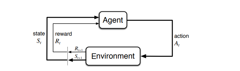
Figure 1. The agent–environment interaction in a Markov decision process. [Source: Sutton & Barto (2018)]
As the decision-maker, the agent repeatedly performs the above process and continuously uses the reward to update its policy in order to maximize the total returns.
The policy $\pi$ of an agent in the Markov Decision Process is defined as:
\[\pi(a\vert s) = \mathbb{P}_\pi[A_t = a\mid S_t = s]\]Value Function
As for the agent, how can it update the policy to obtain the best outcomes? In other words, the agent needs an evaluation method to determine whether the current policy is the optimal solution. In the process of agent-environment interaction, we can see that there is a reward generated at each time-step corresponding to the action chosen by the agent, but the reward cannot be directly used as an evaluation criterion for the policy. This reward can only represent the return of the current step, and the subsequent reward may be completely different. For example, in some chess games, the player can only determine the win or loss at the end of the games and thus receive a reward with a large value, but we can not tell the win or loss according to the reward obtained in the previous rounds. Therefore, a value function that takes into account the current and subsequent rewards should be proposed as an evaluation method.
The state-value function is used to measure how good or bad the state $s$ is under the policy $\pi$. In MDP, the next state $s’$ is only related to the current state $s$ and the action $a$ taken by the agent, so the reward $r$ is also only related to the current state $s$ and action $a$.
So the total sum of discounted future rewards(return) is:
\[G_t=R_{t+1}+\gamma R_{t+2}+\gamma^2R_{t+3}+\cdots=\sum_{k=0}^\infty\gamma^kR_{t+k+1}\]The state-value function is defined as:
\[v_\pi(s)=\mathbb{E}_\pi[G_t\mid S_t=s]\]The action-value function can also be defined in a similar way as:
\[q_\pi(s,a) = \mathbb{E}_\pi[G_t \mid S_t = s,A_t = a]\]Thus we can use these value functions to evaluate the current policy more accurately.
Optimal Value
The agent aims to maximize the total sum of future rewards, thus we define the optimal value function as:
\[v_*(s) = \max_{\pi}v_{\pi}(s) = \max_a q_{\pi^*}(s,a)\]with the optimal action value $q_*(s,a)=\max_\pi q_\pi(s,a)$.
Bellman Equation
The goal of reinforcement learning is to maximize the total rewards of the system, for which we need to introduce the Dynamic Programming Equation, also known as the Bellman Equation. Bellman Equation can be used to discretize the decision problem into smaller subproblems using the dynamic programming method, it can be used to optimize the objective function of reinforcement learning, which is to maximize the return.
The value function can be decomposed into two parts:
- immediate reward $R_{t+1}$
- discounted value of successor state $\gamma v(S_{t+1})$
Then we can derive the recurrence relationship between the value of a state and the values of its successor states for the state-value function:
\[\begin{aligned} v_\pi(s) &= \mathbb{E}_\pi [G_t\mid S_t=s]\\ &=\mathbb{E}_\pi [R_{t+1}+\gamma R_{t+2}+\gamma^2 R_{t+3}+...\mid S_t=s]\\ &=\mathbb{E}_\pi[R_{t+1}+\gamma (R_{t+2}+\gamma R_{t+3}+...)\mid S_t=s]\\ &=\mathbb{E}_\pi[R_{t+1}+\gamma G_{t+1}\mid S_t=s]\\ &=\mathbb{E}_\pi[R_{t+1}+\gamma v_\pi(S_{t+1})\mid S_t=s] \end{aligned}\]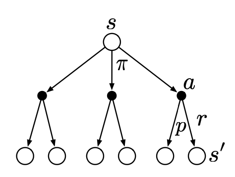
Figure 2. Backup diagram for $v_\pi$[Source: Sutton & Barto (2018)]
Figure 2. Backup diagram for $v_\pi$[Source: Sutton & Barto (2018)]
Fig. 2 shows the relationship between the value of the current state and its next state. $v_\pi(s)$ is a probabilistic sum of all possible pairs of $r + \gamma v_\pi(s’)$.
Similarly, we can obtain the Bellman Equation for the action-value function:
\[\begin{aligned}q_\pi(s, a) &= \mathbb{E}_\pi [R_{t+1} + \gamma v_\pi(S_{t+1}) \mid S_t = s, A_t = a] \\&= \mathbb{E}_\pi [R_{t+1} + \gamma \mathbb{E}_{a\sim\pi} q(S_{t+1}, a) \mid S_t = s, A_t = a]\end{aligned}\]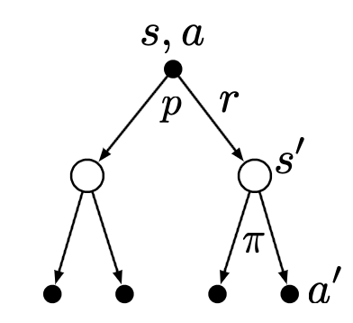
Figure 3. Backup diagram for $q_\pi$ [Source: Sutton & Barto (2018)]
Bellman Expectation
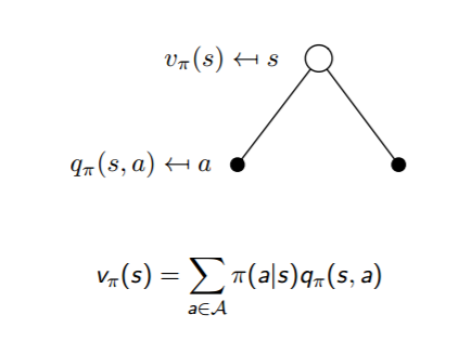
Figure 4. $v_\pi$ short backup diagram
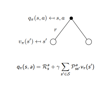
Figure 5. $q_\pi$ short backup diagram
With Figure 2 and Figure 3, we can specifically analyze the transition process between action-value function and state-value function as shown in Figure 4 and Figure 5. So, the equation of the relationship between $v_\pi(s)$ and $q_\pi(s,a)$ is defined as:
\[v_\pi(s)=\sum_{a\in A}\pi(a \vert s)q_\pi(s,a)\] \[q_\pi(s,a)=R^𝑎_𝑠+\gamma\sum_{s'\in S}P^a_{ss'}v_\pi(s')\]Combining the above two equations, we can get:
\[v_{\pi}(s) = \sum\limits_{a \in A} \pi(a\vert s)(R_s^a + \gamma \sum\limits_{s' \in S}P_{ss'}^av_{\pi}(s'))\] \[q_{\pi}(s,a) = R_s^a + \gamma \sum\limits_{s' \in S}P_{ss'}^a\sum\limits_{a' \in A} \pi(a'\vert s')q_{\pi}(s',a')\]These are the Bellman Expectation Equations, which represent the value function in a recursive manner.
Bellman Optimality
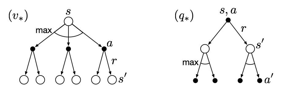
Figure 6. Backup diagrams for $v_*$ and $q_*$ [Source: Sutton & Barto (2018)]
Solving a reinforcement learning problem means that we need to find an optimal policy $\pi$ that makes the agent always obtains a greater or equal return than a policy $\pi’$ for the finite MDPs. In other words, $\pi\geq\pi’$if and only if $v_\pi(s)\geq v_{\pi’}(s)$ for all $s \in S$. This optimal policy is denoted as $\pi_*$.
In general, we find the optimal policy by comparing the value functions of different policies. Similar to the Bellman Expectation Equations, the optimal state-value function can be defined as the largest of the state-value functions of all policies:
\[v_{*}(s) = \max_{\pi}v_{\pi}(s)\]Similarly, the optimal action-value function can be defined as:
\[q_{*}(s,a) = \max_{\pi}q_{\pi}(s,a)\]So for the optimal policy $\pi_*$, based on the optimal action-value function we define as:
\[\pi_{*}(a|s)= \begin{cases} 1 & {\text{if}\;a=\arg\max_{a \in A}q_{*}(s,a)}\\ 0 & {\text{else}} \end{cases}\]This optimal policy $\pi_*$ is the optimal solution to the reinforcement learning problem.
In the Bellman Expectation, we analyze the relationship between the action-value function and the state-value function. So for the Bellman Optimality, we can also get:
\[v_{*}(s) = \max_{a}q_{*}(s,a)\] \[q_{*}(s,a) = R_s^a + \gamma \sum\limits_{s' \in S}P_{ss'}^av_{*}(s')\]Combining the above two equations, we can get:
\[v_{*}(s) = \max_a(R_s^a + \gamma \sum\limits_{s' \in S}P_{ss'}^av_{*}(s'))\] \[q_{*}(s,a) = R_s^a + \gamma \sum\limits_{s' \in S}P_{ss'}^a\max_{a'}q_{*}(s',a')\]Classical Methods
Dynamic Programming(DP)
For dynamic programming, it is mainly to divide a problem into many sub-problems and get the optimal solution for the whole problem by finding the optimal solutions to the sub-problems. It is also possible to derive the state of the whole problem by finding recurrence relations between the states of the sub-problems. These two properties can also be exploited to solve reinforcement learning problems.
Typically, the reinforcement learning problem can be divided into two types:
- Prediction Problem
- Control Problem
Policy Evaluation
To solve the prediction problem of reinforcement learning, DP can be used to compute the state-value function $v_\pi$ for an arbitrary policy $\pi$. This process is generally called Policy Evaluation.
Assuming that we have calculated the values of all the states in the $k$-th iteration, then in the $(k+1)$-th round we can use the state values calculated in the $k$-th round to calculate the state values in the $(k+1)$-th round. By using the Bellman Equation, we can get:
\[\begin{aligned}v_{k+1}(s) &= \mathbb{E}_\pi[R_{t+1}+\gamma v_k(S_{t+1})\mid S_t=s]\\ &= \sum_a \pi(a\vert s)\sum_{s',r}p(s',r \vert s,a)[r+\gamma v_k(s')]\end{aligned}\]Policy Improvement
The value function for selecting $a$ in current $s$ with policy $\pi$ can be computed in Bellman Equation:
\[\begin{aligned}q_\pi(s, a) &= \mathbb{E} [R_{t+1} + \gamma v_\pi(S_{t+1}) \mid S_t=s, A_t=a]\\ &= \sum_{s', r} p(s', r \vert s, a) (r + \gamma v_\pi(s'))\end{aligned}\]The Policy Improvement Theorem suggests that $\pi$ and $\pi’$ can be any pair of deterministic policies, for all $s\in S$ we have:
\[q_\pi(s, \pi'(s))\geq v_\pi(s)\]In this case, the policy $\pi’$ should be better than or equal to the policy $\pi$. With the Bellman Optimality, we can get:
\[v_{\pi'}(s) \geq v_\pi(s)\]To find better policies, we use a greedy policy to choose the action that appears best according to the value of $q_\pi(s,a)$.
Policy Iteration
To solve the control problem in reinforcement learning, we use Generalized **Policy Iteration(GPI) to repeatedly improve the policy according to the state value of a deterministic policy.
In the process of GPI, the first step is to compute the state-value $v_{\pi_i}$ of the current policy $\pi_i$ using policy evaluation. Second, update the policy $\pi_i$ according to the state-value $v_{\pi_i}$ using policy improvement, then return to the first step and keep iterating to obtain the converged optimal policy $\pi_∗$ and the state value $v_∗$:
\[\pi_0 \xrightarrow[]{\text{E}} v_{\pi_0} \xrightarrow[]{\text{I}}\pi_1 \xrightarrow[]{\text{E}} v_{\pi_1} \xrightarrow[]{\text{I}}\pi_2 \xrightarrow[]{\text{E}} \dots \xrightarrow[]{\text{I}}\pi_* \xrightarrow[]{\text{E}} v_*\]where $\xrightarrow[]{\text{E}}$ denotes a policy evaluation and $\xrightarrow[]{\text{I}}$ denotes a policy improvement.
Value Iteration
Unlike the policy iteration, the value iteration does not need to wait for the exact convergence of the state values before adjusting the policy but adjusts the policy as the state values iterate. In this case, we can reduce the number of iterations and the update rule becomes:
\[\begin{aligned}v_{k+1}(s) &= \max_{a \in A}\mathbb{E}[R_{t+1}+\gamma v_k(S_{t+1})\mid S_t=s,A_t=a]\\ &= \max_{a \in A}\sum_{s', r} p(s', r \vert s, a) (r + \gamma v_k(s'))\end{aligned}\]Summary
- $V(S_t)\leftarrow E_\pi[R_{t+1}+\gamma V(S_{t+1})]=\sum_{a}\pi(a\vert S_t) \sum_{s',r}p(s',r\vert S_t,a)[r+\gamma V(s')]$
- The expected values are provided by a model. But we use a current estimate $V(S_{t+1})$ of the true $v_π(S_{t+1})$.
- Model based: model in DP is a mathematical representation of a real-world process. It requires a complete and accurate model of the environment. It requires all the previous states.
- Bootstrapping: update the value of the current state using an estimated value of subsequent states.
Monte Carlo
The Monte Carlo(MC) method estimate the true value of a state by sampling a number of state from complete episodes. A complete sequence means that the sequence has to reach the terminate state and a complete sequence following a given policy $\pi$ is:
\[S_1,A_1,R_2,S_2,A_2,...S_t,A_t,R_{t+1},...R_T, S_T\]The dynamic programming approach requires a model $p(s’,r\vert s,a)$ when calculating the value function of the state, whereas, the model-free Monte Carlo method does not depend on the model state transition probabilities, and it learns empirically from the complete sequences of states.
\[G_t =R_{t+1} + \gamma R_{t+2} + \gamma^2R_{t+3}+... \gamma^{T-t-1}R_{T}\]In the Monte Carlo method, we update the value of states or action-state pairs based on the average return $v(s)$ we experienced when after visiting the state $s$.
The same state $s$ may occur multiple times in an episode. To estimate the return, there are two MC methods: the first-visit method only estimates $v_\pi(s)$ when we first visit the state $s$ in the episode as the average of the returns; while the every-visit method is to calculate the average of every visit through the state in a given episode.
Monte Carlo Control
The idea is similar to generalized policy iteration(GPI). In MC, the policy evaluation method and estimation of value functions are different from those in DP.
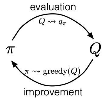
Figure 7. Monte Carlo version of policy iteration
The policy iteration in MC starts with a random policy $\pi_0$ and ends with the optimal policy $\pi_\ast$ and the optimal action-value function $q_\ast$(Figure 7).
\[\pi_0 \xrightarrow[]{\text{E}} q_{\pi_0} \xrightarrow[]{\text{I}}\pi_1 \xrightarrow[]{\text{E}} q_{\pi_1} \xrightarrow[]{\text{I}}\pi_2 \xrightarrow[]{\text{E}} \dots \xrightarrow[]{\text{I}}\pi_* \xrightarrow[]{\text{E}} q_*\]Since MC is a model-free approach, it makes more sense to estimate the action value, thus the policy evaluation in MC is supposed to estimate $q_\pi(s,a)$. Both the first-visit method and every-visit method need to calculate the average of the returns. Specifically, the incremental update method is used to calculate the average value when iterating through each state:
\[Q(s,a)=Q(s,a)+\frac{1}{N(s,a)}\left( G_{t}-Q(s,a) \right)\]As for policy improvement in MC, we use greedy policy based on current value function. In this case, the greedy policy for every action-value function $Q(s,a)$ is:
\[\pi(s)=\argmax_a Q(s,a)\]Summary
- $V(S_t)\leftarrow V(S_t)+\alpha(G_t-V(S_t))$
- $G_t$ is the target: the actual return after time $t$
- Model-free: It requires only experience such as sample sequences of states, actions, and rewards from online or simulated interaction with an environment. But requires no prior knowledge of the environment.
- No bootstrapping
- Sampling: update does not involve an expected value and sampling average returns approximate expectation $v_\pi$
Temporal-Difference Learning
The Temporal-Difference(TD) Learning combines the experience sampling with Bellman equations. Similar to the Monte Carlo Method, TD learning also is a model-free method. TD method also combines some of the ideas in DP, it updates the current estimate based on the estimates of the learned value functions(bootstrapping), without waiting for the end of the entire episode.
A simple every-visit Monte Carlo method for updating the value function can be represented as:
\[V(S_t)\leftarrow V(S_t)+\alpha[G_t-V(S_t)]\]where $G_t$ is the return at time $t$, and $\alpha$ is a constant step-size parameter. This means that in MC, we have to wait until the end of the episode to get the actual return value.
Whereas, in temporal-difference learning, we use bootstrapping to update the value estimate according to the value estimate of the successor state and the new observed reward. The update rule for the TD method is:
\[V(S_t)\leftarrow V(S_t)+\alpha[R_{t+1}+\gamma V(S_{t+1})-V(S_t)]\]where $R_{t+1}+\gamma V(S_{t+1})$ is the TD Target, and the difference between estimated value of $S_t$ and the better estimate $R_{t+1}+\gamma V(S_{t+1})$ is the TD Error. This TD method is called TD(0), or one-step TD.
Similarly, the update rule of action-value estimation is:
\[\begin{aligned}Q(S_t, A_t) &\leftarrow Q(S_t, A_t) +\alpha[G_t - Q(S_t, A_t) ]\\ &\leftarrow Q(S_t, A_t) +\alpha[R_{t+1}+\gamma Q(S_{t+1}, A_{t+1}) - Q(S_t, A_t) ]\end{aligned}\]Summary
- TD(0): $V(S_t)\leftarrow V(S_t)+\alpha(R_{t+1}+\gamma V(S_{t+1})-V(S_t))$
- $R_{t+1} + \gamma V(S_{t+1})$ is the target: an estimate of the return
- it is an estimate like MC target because it samples the expected value
- it is an estimate like the DP target because it uses the current estimate of $V$ instead of $v_\pi$
- Combine both: Sample expected values and use a current estimate $V(S_{t+1})$ of the true $v_\pi(S_{t+1})$
- Both bootstrapping and sampling, model-free
SARSA
SARSA algorithm is a method for solving reinforcement learning control problems using Temporal-Difference Learning and it is an on-policy TD control method. The name of the SARSA algorithm is composed of the letters S,A,R,S,A. And S,A,R,S,A stand for $(S_t, A_t, R_{t+1}, S_{t+1}, A_{t+1})$ in the episode respectively. The process is shown as follows (Figure 8):
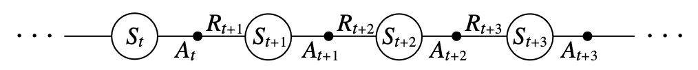
FFigure 8. An episode consists of an alternating sequence of states and state–action pairs
In the iteration, we first select an action $𝐴’$ according to the current state $S$ using the $\epsilon$-greedy policy. So that the system will move to a new state $S’$, while giving us an immediate reward $R$. And in the new state $S’$ we will select an action $A’$ from the state $S’$ also using the $\epsilon$-greedy policy, but note that at this point we do not execute this action $A’$, but only use it to update our value function.
Note: the step size $\alpha$ needs to decay as the iterations proceed so that the action-value function $Q$ can converge. When $Q$ converges, the $\epsilon$-greedy policy also converges to optimality.
Summary
- Given a State, we select an Action, observe the Reward and subsequent State, and then select the next Action according to the current policy
- The target is the reward returns plus the discounted value of the next state-action pair: $R_{t+1}+\gamma Q(S_{t+1},A_{t+1})$
- SARSA learns the action-value function, the update rule: $Q(S_t,A_t)\leftarrow Q(S_t,A_t)+\alpha[R_{t+1}+\gamma Q(S_{t+1},A_{t+1})-Q(S_t,A_t)]$
- On-policy: selecting actions only according to the current policy
In the SARSA algorithm, we constantly evaluate the value $Q_\pi$ of the policy $\pi$, while at the same time the policy $\pi$ is updated (using the greedy method) according to the value function. Thus, SARSA has the same policy before(select new action) and after(update value function), which is the main idea of on-policy.
Q-Learning
Unlike SARSA, the Q-Learning algorithm is an off-policy TD control method. Q-learning uses two different control policies, first using the $\epsilon$-greedy method to select new actions. While, unlike SARSA, for the update of the value function, Q-learning uses a greedy policy instead of the $\epsilon$-greedy method.
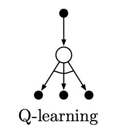
Figure 9. The backup diagram for Q-learning
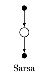
Figure 10. The backup diagrams for SARSA(0)
First, we select action $A$ based on state $S$ using the $\epsilon$-greedy method, then execute action $A$ to get reward $R$ and move to the next state $S’$. Then select $A’$ according to the state $S’$ using the greedy method, which means that selecting the action $𝑎$ as $A’$ maximizes $Q(S’,a)$ to update the value function. The update rule of Q-learning is defined as:
\[Q(S_t, A_t) \leftarrow Q(S_t, A_t) + \alpha (R_{t+1} + \gamma \max_{a \in \mathcal{A}} Q(S_{t+1}, a) - Q(S_t, A_t))\]As shown in Figure 9, choose the one that maximizes $Q(S’,a)$ as $A’$ among all three black circle actions at the bottom of the figure. The selected action will only be used in the update of the value function and will not be executed at this point.
Summary
- Q-learning choose action greedily with respect $Q(s,a)$
- Q-learning approximates optimal action value function $q_\ast(s,a)$, the update rule: $Q(S_t,A_t)\leftarrow Q(S_t,A_t)+\alpha[R_{t+1}+\gamma\displaystyle\max_aQ(S_{t+1},a)-Q(S_t,A_t)]$
- Off-policy: taking the best action when bootstrapping
Expected SARSA
When the SARSA algorithm changes the form of the update to use the expectation of $Q(s,a)$, it makes the SARSA algorithm into an off-policy algorithm, called Expected SARSA. The update rule is as follows:
\[\begin{aligned}Q(S_t,A_t)&\leftarrow Q(S_t,A_t)+ \alpha [R_{t+1} +\gamma\mathbb{E}_\pi [Q(S_{t+1} ,A_{t+1})\mid S_{t+1} ]-Q(S_t,A_t)]\\ &\leftarrow Q(S_t,A_t)+ \alpha [R_{t+1} +\gamma\sum_a\pi(a\vert S_{t+1}) Q(S_{t+1} ,a)-Q(S_t,A_t)]\end{aligned}\]This method increases the computational complexity compared to the original SARSA algorithm but relatively reduces the variance due to the random selection of $A_{t+1}$.
Deep Q-Network
Whether it is dynamic programming, Monte Carlo methods, or temporal-difference learning, the states are discrete finite sets of states $\mathcal{S}$. However, when the state and action space are large, methods like Q-learning cannot memorize a huge Q-Table.
So a feasible way is to approximate the value function. This method introduces both a state value function $V$ and a parameter $\theta$ to approximate the values. It takes state $s$ as input, which is calculated to estimate the value of state $s$:
\[\hat{V}(s;\theta)\approx V_\pi(s)\]Similarly, for an action-value function $Q$:
\[\hat{Q}(s,a;\theta) \approx Q_{\pi}(s,a)\]The Deep Q-Learning algorithm is derived from Q-Learning. Deep Q-learning calculates the Q value by the neural network or Q-network in this case. Generally, this method is referred to as Deep Q-Network(DQN).
The main mechanism used by DQN is Experience Replay, which stores the rewards $R$ and states $S$ in a replay memory from each interaction with the environment. Then DQN uses them to update the target Q value.
The target Q value obtained from Experience Replay and the Q value calculated through the Q network may have an error. Then we can update the parameters of the neural network by back-propagation of the gradient $\theta$, when $\theta$ converges, we can get the method to approximate the Q value.
References
- Sutton, Richard S., and Andrew G. Barto. Reinforcement learning: An introduction . MIT press, 2018.
- Li, Yuxi. “Deep reinforcement learning: An overview.” arXiv preprint arXiv:1701.07274 (2017).
- Silver, David. “Introduction to reinforcement learning with david silver.” DeepMind x UCL (2015).
- Salimans, Tim, et al. “Evolution strategies as a scalable alternative to reinforcement learning.” arXiv preprint arXiv:1703.03864 (2017).
- Mnih, Volodymyr, et al. “Playing atari with deep reinforcement learning.” arXiv preprint arXiv:1312.5602 (2013).